During our last discussion of building simple formulas we kept our work to one worksheet. This tutorial will carry the exercise one step further by linking two different sheets in a formula so that the information in one sheet is completely dependent on the other and that by updating the original sheet to meet your immediate needs; you are also completing another task that is on the horizon. This will become apparent as we move forward through this lesson. This lesson will also come with an added bonus as in addition to formulas you will also learn to format a table with borders and colors to make it attractive and easily readable. By the end of this lesson you will be able to do the following:
- Rename a sheet to identify its purpose, task, or intention
- Refer to another sheet to gather data necessary in your active sheet.
- Apply formats like color, borders, bold font, italic font, etc. to a range of cells.
- Calculate totals to include sales tax for replenishing your inventory.
- Merge a range of cells to create one cell that stretches across several columns/rows.
- Insert a formula that will automatically enter the date so that when you print the form it will automatically have the current date on it.
- Insert rows
- Resize columns
In our previous lesson, if you caught it, you completed the practice imaged below; you’ll need to retrieve it from your computer or from the grab box at the bottom of this screen, it is titled ‘Linking Worksheets.’ If you did not and you would like to complete it to catch up you may do so at: Understanding and Building Simple Formulas . If you’d rather begin from here, you can simply download and save the file titled ‘Linking Worksheets’ located in the grab box at the bottom of this screen. While you are down there, feel free to turn on some Christmas music to enjoy while you complete this exercise. You'll find it to the right of the grab box.
Three fundamental and important rules as we go through this tutorial are: 1. Read each instruction fully before performing as each step has hints to keep you on track and if you try to do as you read you may get ahead of yourself and end up off track and frustrated; so read first, then perform (as you read again if necessary), but always read the instruction before performing. 2. Do only what the instructions say and nothing more, more could take you off track. Something as simple as striking an enter key by mistake can take you off course. 3. If you do make such a mistake perform the following steps to undo and start over with the object again: a. Hold down your Ctrl key, b. strike the Z key, c. and then release the Ctrl key. This will undo you last move. I give you this process because it works in all versions of Excel for as far back as I can remember. Other ways of making this same function occur differ from one version to another. If you know them already, great. Now, having covered your safeguards for this lesson, let’s begin. Once you have downloaded and opened the file named Linking Worksheets located in the grab box at the bottom of this screen, you should see what looks like the image below. Do you see it? Notice the tab of the sheet at the bottom left corner of the screen labeled ‘Sheet1.’ We want to rename this sheet to ‘Sales’ to reflect its purpose, to calculate sales and gain/losses. 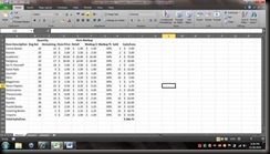 To do this, perform the following instructions: 1. Point to and double click the sheet tab so that it highlights the tab name as you see in the image below. If double clicking is difficult for you, you can also right click and then select ‘Rename’ from the list of options in the menu that appears when you right click. Either method will result in the tab label being highlighted as you see below.
  2. Once you have successfully highlighted the sheet tab, type ‘Sales’ and strike the ‘Enter’ key to rename the sheet.
  3. The work we will be performing today will be primarily in Sheet2, but first we are going to rename it to ‘Requisition.’ Click that tab to make that sheet active.
  4. Now repeat steps (1) and (2) to rename Sheet2 to ‘Requisition.’
  5. Now we are going to pick up data from the Sale sheet to display and automatically update in the Requisition sheet. Click on cell A1 on your Requisition sheet to make it active, if you are unclear on how to get there or what this ‘A1’ is, you’ll need to go through the tutorial Understanding and Building Simple Formulas first, and then come back to this lesson.
  6. Strike your = key
  7. Point to and click on the Sales tab and then point to and click cell A1 of your Sales sheet. It should then have a scrolling marque around the cell as seen below. Also, make a mental note that the data in the sheet reaches as far down as row 20; you’ll need to know this in step 11.
  8. Strike the ‘Enter’ key. A ‘0’ will appear in A1 of the Requisition sheet because, as you will recall, there was nothing entered into the A1 cell of the Sales sheet.
  9. Point to and click cell A1 of the Requisition sheet to make it active.
  10. Recall in our last lesson that we performed what is called a fill-down. Notice in the image below that at the lower right corner of the cell there is a small square; known as the ‘fill-handle.’
 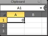 11. Point to this square until your cursor becomes a small, bold plus sign; when it does press and hold your left mouse button and drag down until you reach and include row 20, see below. Recall that in step 7 we made a mental note that the data in the Sales sheet reached row 20.
  12. Once you have reached row 20 release the mouse button you are holding and watch as the data from the Sales sheet appears in the selected range on the Requisition sheet, see below.
  13. Notice that the data spills beyond the right border of the cells. This is a simple fix. Simply complete the following steps (keep the cells highlighted, don’t click inside the sheet or it will deselect, if you do so by mistake you can simply highlight them again before performing step 14) a. Notice that there is a line between the column A and column B indicators.
  b. Position your cursor over this line until it becomes a vertical line with an arrow in the middle of the line pointing both to the right and the left. c. Double click and it will automatically resize to fit the longest item in the list held in the column on the left side of the click (in this case column A)
  14. With cells A1:A20 highlighted point use the fill-handle to fill in across the next two columns. See below. (Now any time you update these items on the Sales sheet it will also update on the Requisition sheet.)
 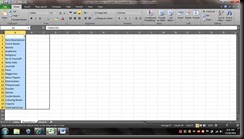 15. Notice that now Requisition rang A1:C20 now hold the data entered in the same range of the Sales sheet.
  16. Make cell D2 of your Requisition sheet active and type in that cell Requisition; strike your ‘Enter’ key. This column will calculate how many items you need to requisition for purchase to your purchasing department or business office.
  17. Fill in the remaining columns accordingly: E2 should be Item Cost (what each item cost you to purchase at “retail” value) F2 should be Item Expense (this will calculate the total expense for replenishing this item on your shelf.
  18. Now we will begin our formulas for these three columns. Make D3 your active cell and strike your ‘Enter’ key.
  19. Point to and click cell B3, you screen should look like the image below
 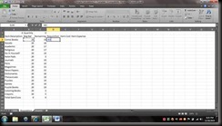 20. Strike you – key and point to and click cell C3 (this will subtract the value of C3 from the value of B3)
  21. Strike you ‘Tab’ key (this will finalize your formula in cell D3 and place you in cell E3 making it your active cell); then strike your = key (see below)
  22. Point to and click your Sale tab and then point to and click cell E3 in the Sales sheet (there’s that marque again so you can confirm that you selected the cell you intended)
  23. Strike the ‘Tab’ key. Again this finalizes the formula in the E3 cell of your Requisition sheet and makes cell F3 active for its formula. (Notice that it also brought the retail value over from the Sales sheet to the Requisition sheet, now when this information is updated on the Sales sheet it will also update on the Requisition sheet)
  24. With cell F3 active strike the = key
  25. Point to and click cell D3
  26. Strike the * key
  27. Point to and click cell D3 (this will multiply the item cost and the number of items to requisition to reveal the total expense for replenishing that item on your shelves)
  28. Strike the ‘Tab’ key to finalize your formula in cell F3.
  29. Now we want to fill down the other rows. Select range D3:F3 as indicated below.
 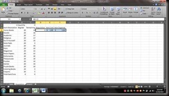 30. Use your fill-handle to fill down to row 20.
  31. Once you release the button after the fill down your sheet should look like the one below.
 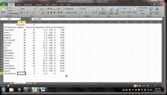 32. Now to figure our total cost for restocking our shelves. Select range B20:F20 as seen below.
  33. Strike the ‘Delete’ key to clear its contents
 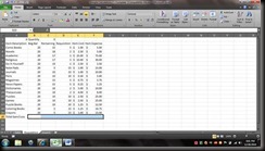 34. Make cell F20 active
  35. Locate the AutoSum feature on your tool bar; it should look similar to the highlighted item in the image below
  36. Once you have located it, double click on it. Notice that the first click places the marque around the cells directly adjacent and above the active cell.
  37. On the second click it will reveal the results of your double click with a value that represents the sum of the above values
  38. Of course, we all have to pay taxes so this is not a complete representation of our total cost of restocking. First let’s rename that row from ‘Total Gain/Loss’ to ‘SubTotal.’ Make cell A20 active and type the word ‘SubTotal.’
  39. Below that, in cell A21 type tax
  and in cell A22 type Total Expense
 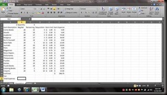 40. In cell B21 we need to note what kind of tax will be required (.07, .08) depending on the sales tax of the state you live in. In this case we are going to use a 7 percent sales tax by entering .07 in cell B21
  41. Next we are going to figure how much sales tax this purchase will cost us. Make cell F21 active and strike the = key
  42. Point to and click cell F20
 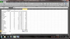 43. Strike the * key
  44. Point to and click cell B21 to multiply your subtotal and your sales tax
 requirement to find your tax cost.
  45. Strike the ‘Enter’ key to finalize the formula and make the cell below it (F22) active. Notice that this purchase will result in a sales tax
 expense of 18.67. Strike the = key
  46. Point to and click cell F20
  47. Strike the + key
  48. Point to and click cell F21
  49. Strike the ‘Enter’ key. Notice that your total purchase will cost you $285.42.
  50. Such a sheet can be, not to mention boring, but easily misread without any boundaries or guides. So we will use some formatting features to change this and make this sheet much more professional in appearance when presenting to another department. Let’s begin with bolding and italicizing some key bits of focus information in our spreadsheet. We want to bold our SubTotal row, our Total row, and our column heading row. Point to and click row indicator 20
  51. Locate the Bold button on the toolbar as seen below
 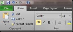 52. Once you have located it, click it. The text in the selected row becomes a bold, heavy type font.
 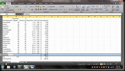 53. Repeat this same step to bold the Total Expenses row (indicator for row 22)
  54. Highlight row 21 by clicking on the indicator of row 21
  55. Locate the Italic button on the toolbar as seen below
  56. Once you have located it, click it. The text in the selected row leans to the right slightly giving it an italic appearance.
  57. Next we will add some borders that will further separate the focus information from the focus dependent information and give the table boundaries. Select range A3:F19
  58. Locate the borders tool on your toolbar and click on the small arrow pointing downward at the right of the border button as seen below:
  59. Once you have located it, click the arrow pointing down to reveal the menu you see below. Left click on the highlighted option you see below called Outside Borders (if you have screen tips turned on you can see the short cut for making this command occur – in this case it is Ctrl+Shift+& [See Keys to Faster MS Office Operations and Document Navigation to learn out how to execute/use these shortcut keys])
  60. Once you click on Outside Borders, click outside the selected range to view the border you have just placed.
  61. Select range A2:F22
 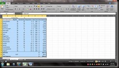 62. Locate the same Border button on your toolbar and click on the same arrow. This time click on the Thick Box Border option. See below.
  63. Click off the selection to view the border you have just placed
  64. Now we are going to apply some color to our sheet. Select range A22:F22
 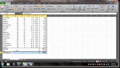 65. Locate the border button on your toolbar again and click on the arrow. This time click on the Top Border option.
  66. Now locate the color fill button on your tool bar and click on its arrow (looks like a tipped paint can) Pick a color and click on it, I’m choosing yellow, a bright and cheerful color.
  67. Now click off the selection to view the formats you have applied.
  68. Now select range A2:F2 and repeat step 66 to apply your color to this range.
  69. Click of this range to view the color you have just applied.
  70. Now recall that row 1 held formulas that provided no real asset to this spread sheet so we can delete it. Select row 1 by clicking on its indicator.
  71. Strike your ‘Delete’ key.
  72. Now a purchaser may not necessarily need to know how many you sold or what your base inventory should be so columns B and C are solely for operational purposes only and only serve as unnecessary data to the recipient. Thus there is no need in it being present or seen when submitted to the purchaser. But to completely remove it would totally destroy everything we have just accomplished. So to remove it from sight without removing it from the sheet we will perform these steps. Point to the B column indicator; press and hold the left mouse button; drag to the right through until both B and C columns are highlighted, as seen below, and then release the left mouse button
  73. Right click on either the B or the C column indicator to reveal the options below. Left click on the ‘Hide’ option.
  74. Click off to the side to deselect the hidden columns and see your table without the columns. (Remember that the B & C columns are completely dependent on the information in the Sales sheet, so you will never have to edit them because every time you make changes to the B or C column in the Sales sheet, it automatically updates on the Requisition sheet; which in turn updates the rest of the Requisition sheet. Give it a try when we are done.)
  Now our form needs a title, and like most forms, a date is a must. Let’s give our form a title and a date command. 75. Make cell A1 active
  76. Select range A1:F1
  77. Locate the ‘Merge and Center’ button on your toolbar as shown below
  78. Click on it to merge cells A1:F1 into one cell that stretches across the columns highlighted A-F. The same can be done in rows or the combination of rows and columns. Notice how A1:F1 merged to form one cell.
  79. With that cell still highlighted/selected type ‘Inventory Requisition’
  80. We now need to insert a row between the form’s title and the form’s table. Click on row indicator 2 to highlight row two
 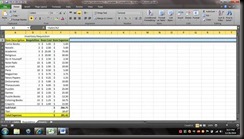 81. Right click on row indicator two to reveal the options shown below
  82. Left click on ‘Insert.’ Notice a new row appears above the row you selected prior to the insert.
  83. But this move left an unwanted border at the bottom of the cell holding the form’s title. Select the cell holding the form’s title
  84. Locate the border button on the toolbar and click on the arrow button. Click on the ‘No Border’ option to remove the border from the form title
 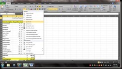 85. Select cells A2:F2
  86. Repeat steps 77 and 78 to merge these cells. This will hold our automatic date
 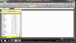 87. With this newly merged cell still active, locate the ‘Insert Function’ button on the formula bar, located right under your toolbar and to the right of the name box. See below.
 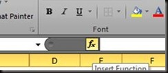 88. Once you locate it, click on it to reveal the dialog box below. Notice that a selection of text is highlighted in the box.
  89. With the text selected, type ‘date’ and notice that the selected text is immediately replaced with the word ‘date.’ Click the ‘Go’ button or strike the ‘Enter’ key. Notice that the list in the section below where the text was at changes (see below).
  90. Point to and click the “NOW” option. Click the ‘OK’ button. You’ll notice a box appear like the one below. Click OK.
  91. Notice that the current date and time is entered into the form. Each time you open this workbook the date automatically updates.
 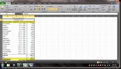 Each time you conduct your monthly inventory and determine your Gain/Loss on the sales sheet, you will automatically be completing your monthly Requisition. All you have to do is click on the requisition sheet, print, and submit. At the start of the next month when you’ve restocked your shelves, you’ll replace the data in the Remaining Balance column of your Sales sheet with the a number matching the beginning balance only to do it all again when inventory and order time hits again. Considering the positive feedback on the tutorial Understanding and Building Simple Formulas, I hope you guys enjoy this one just as much. Here's a hint as to what to look forward to. What to look forward to… At some point we can come back and build a macro button that will automatically reset the form for you. But, we’ll leave that for another time. I’m also looking forward to showing you how to generate a pie chart to show the percentage of sales per item which is useful in identifying where your sales were strongest during the month. Maybe later we can look forward to extending this to showing trends that will show when during a year your sales seem to be at their highest in order to predict a higher sales rate, a higher need for materials, and consequently a higher inventory count. On another note… I have a couple of announcements to make regarding my blog, I’ve recently invited a co-writer to join my blog in publishing such post as these. He may be contributing in the near future. So we can look forward to the possibility of more input, more tutorials, and a broader range of IT topics. I’d like to introduce you to a new page (Sweet IT Deals) that I’ve added to my blog where I discuss great deals I find online. Each item is compared to other popular venders and the advantage is discussed. I only present them if they are a benefit or savings in comparison to your local/popular vendor. And, yes, you’ll likely find IT items posted there for the most part; maybe the occasional other items, depending on the season. I sincerely hope that I’ve kept them simple enough without boring you. I do try to post a balance of the two. On some occasions a more advanced tutorial and at other times a beginners tutorial. So if I don’t get back to the topic you are looking forward to, keep an eye out because its coming. Don’t forget you can always subscribe for alerts to notify you of updates and can rate my posts and add a comments by replying to my posts. I always look forward to hearing from my readers. Thank you for stopping by.
 To do this, perform the following instructions: 1. Point to and double click the sheet tab so that it highlights the tab name as you see in the image below. If double clicking is difficult for you, you can also right click and then select ‘Rename’ from the list of options in the menu that appears when you right click. Either method will result in the tab label being highlighted as you see below.
  2. Once you have successfully highlighted the sheet tab, type ‘Sales’ and strike the ‘Enter’ key to rename the sheet.
  3. The work we will be performing today will be primarily in Sheet2, but first we are going to rename it to ‘Requisition.’ Click that tab to make that sheet active.
  4. Now repeat steps (1) and (2) to rename Sheet2 to ‘Requisition.’
  5. Now we are going to pick up data from the Sale sheet to display and automatically update in the Requisition sheet. Click on cell A1 on your Requisition sheet to make it active, if you are unclear on how to get there or what this ‘A1’ is, you’ll need to go through the tutorial Understanding and Building Simple Formulas first, and then come back to this lesson.
  6. Strike your = key
  7. Point to and click on the Sales tab and then point to and click cell A1 of your Sales sheet. It should then have a scrolling marque around the cell as seen below. Also, make a mental note that the data in the sheet reaches as far down as row 20; you’ll need to know this in step 11.
  8. Strike the ‘Enter’ key. A ‘0’ will appear in A1 of the Requisition sheet because, as you will recall, there was nothing entered into the A1 cell of the Sales sheet.
  9. Point to and click cell A1 of the Requisition sheet to make it active.
  10. Recall in our last lesson that we performed what is called a fill-down. Notice in the image below that at the lower right corner of the cell there is a small square; known as the ‘fill-handle.’
  11. Point to this square until your cursor becomes a small, bold plus sign; when it does press and hold your left mouse button and drag down until you reach and include row 20, see below. Recall that in step 7 we made a mental note that the data in the Sales sheet reached row 20.
  12. Once you have reached row 20 release the mouse button you are holding and watch as the data from the Sales sheet appears in the selected range on the Requisition sheet, see below.
  13. Notice that the data spills beyond the right border of the cells. This is a simple fix. Simply complete the following steps (keep the cells highlighted, don’t click inside the sheet or it will deselect, if you do so by mistake you can simply highlight them again before performing step 14) a. Notice that there is a line between the column A and column B indicators.
  b. Position your cursor over this line until it becomes a vertical line with an arrow in the middle of the line pointing both to the right and the left. c. Double click and it will automatically resize to fit the longest item in the list held in the column on the left side of the click (in this case column A)
  14. With cells A1:A20 highlighted point use the fill-handle to fill in across the next two columns. See below. (Now any time you update these items on the Sales sheet it will also update on the Requisition sheet.)
  15. Notice that now Requisition rang A1:C20 now hold the data entered in the same range of the Sales sheet.
  16. Make cell D2 of your Requisition sheet active and type in that cell Requisition; strike your ‘Enter’ key. This column will calculate how many items you need to requisition for purchase to your purchasing department or business office.
  17. Fill in the remaining columns accordingly: E2 should be Item Cost (what each item cost you to purchase at “retail” value) F2 should be Item Expense (this will calculate the total expense for replenishing this item on your shelf.
  18. Now we will begin our formulas for these three columns. Make D3 your active cell and strike your ‘Enter’ key.
  19. Point to and click cell B3, you screen should look like the image below
  20. Strike you – key and point to and click cell C3 (this will subtract the value of C3 from the value of B3)
  21. Strike you ‘Tab’ key (this will finalize your formula in cell D3 and place you in cell E3 making it your active cell); then strike your = key (see below)
  22. Point to and click your Sale tab and then point to and click cell E3 in the Sales sheet (there’s that marque again so you can confirm that you selected the cell you intended)
  23. Strike the ‘Tab’ key. Again this finalizes the formula in the E3 cell of your Requisition sheet and makes cell F3 active for its formula. (Notice that it also brought the retail value over from the Sales sheet to the Requisition sheet, now when this information is updated on the Sales sheet it will also update on the Requisition sheet)
  24. With cell F3 active strike the = key
  25. Point to and click cell D3
  26. Strike the * key
  27. Point to and click cell D3 (this will multiply the item cost and the number of items to requisition to reveal the total expense for replenishing that item on your shelves)
  28. Strike the ‘Tab’ key to finalize your formula in cell F3.
  29. Now we want to fill down the other rows. Select range D3:F3 as indicated below.
  30. Use your fill-handle to fill down to row 20.
  31. Once you release the button after the fill down your sheet should look like the one below.
  32. Now to figure our total cost for restocking our shelves. Select range B20:F20 as seen below.
  33. Strike the ‘Delete’ key to clear its contents
  34. Make cell F20 active
  35. Locate the AutoSum feature on your tool bar; it should look similar to the highlighted item in the image below
  36. Once you have located it, double click on it. Notice that the first click places the marque around the cells directly adjacent and above the active cell.
  37. On the second click it will reveal the results of your double click with a value that represents the sum of the above values
  38. Of course, we all have to pay taxes so this is not a complete representation of our total cost of restocking. First let’s rename that row from ‘Total Gain/Loss’ to ‘SubTotal.’ Make cell A20 active and type the word ‘SubTotal.’
  39. Below that, in cell A21 type tax
  40. In cell B21 we need to note what kind of tax will be required (.07, .08) depending on the sales tax of the state you live in. In this case we are going to use a 7 percent sales tax by entering .07 in cell B21
  41. Next we are going to figure how much sales tax this purchase will cost us. Make cell F21 active and strike the = key
  42. Point to and click cell F20
  43. Strike the * key
  44. Point to and click cell B21 to multiply your subtotal and your sales tax
 45. Strike the ‘Enter’ key to finalize the formula and make the cell below it (F22) active. Notice that this purchase will result in a sales tax
 46. Point to and click cell F20
  47. Strike the + key
  48. Point to and click cell F21
  49. Strike the ‘Enter’ key. Notice that your total purchase will cost you $285.42.
  50. Such a sheet can be, not to mention boring, but easily misread without any boundaries or guides. So we will use some formatting features to change this and make this sheet much more professional in appearance when presenting to another department. Let’s begin with bolding and italicizing some key bits of focus information in our spreadsheet. We want to bold our SubTotal row, our Total row, and our column heading row. Point to and click row indicator 20
  51. Locate the Bold button on the toolbar as seen below
  52. Once you have located it, click it. The text in the selected row becomes a bold, heavy type font.
  53. Repeat this same step to bold the Total Expenses row (indicator for row 22)
  54. Highlight row 21 by clicking on the indicator of row 21
  55. Locate the Italic button on the toolbar as seen below
  56. Once you have located it, click it. The text in the selected row leans to the right slightly giving it an italic appearance.
  57. Next we will add some borders that will further separate the focus information from the focus dependent information and give the table boundaries. Select range A3:F19
  58. Locate the borders tool on your toolbar and click on the small arrow pointing downward at the right of the border button as seen below:
  59. Once you have located it, click the arrow pointing down to reveal the menu you see below. Left click on the highlighted option you see below called Outside Borders (if you have screen tips turned on you can see the short cut for making this command occur – in this case it is Ctrl+Shift+& [See Keys to Faster MS Office Operations and Document Navigation to learn out how to execute/use these shortcut keys])
  60. Once you click on Outside Borders, click outside the selected range to view the border you have just placed.
  61. Select range A2:F22
  62. Locate the same Border button on your toolbar and click on the same arrow. This time click on the Thick Box Border option. See below.
  63. Click off the selection to view the border you have just placed
  64. Now we are going to apply some color to our sheet. Select range A22:F22
  65. Locate the border button on your toolbar again and click on the arrow. This time click on the Top Border option.
  66. Now locate the color fill button on your tool bar and click on its arrow (looks like a tipped paint can) Pick a color and click on it, I’m choosing yellow, a bright and cheerful color.
  67. Now click off the selection to view the formats you have applied.
  68. Now select range A2:F2 and repeat step 66 to apply your color to this range.
  69. Click of this range to view the color you have just applied.
  70. Now recall that row 1 held formulas that provided no real asset to this spread sheet so we can delete it. Select row 1 by clicking on its indicator.
  71. Strike your ‘Delete’ key.
  72. Now a purchaser may not necessarily need to know how many you sold or what your base inventory should be so columns B and C are solely for operational purposes only and only serve as unnecessary data to the recipient. Thus there is no need in it being present or seen when submitted to the purchaser. But to completely remove it would totally destroy everything we have just accomplished. So to remove it from sight without removing it from the sheet we will perform these steps. Point to the B column indicator; press and hold the left mouse button; drag to the right through until both B and C columns are highlighted, as seen below, and then release the left mouse button
  73. Right click on either the B or the C column indicator to reveal the options below. Left click on the ‘Hide’ option.
  74. Click off to the side to deselect the hidden columns and see your table without the columns. (Remember that the B & C columns are completely dependent on the information in the Sales sheet, so you will never have to edit them because every time you make changes to the B or C column in the Sales sheet, it automatically updates on the Requisition sheet; which in turn updates the rest of the Requisition sheet. Give it a try when we are done.)
  Now our form needs a title, and like most forms, a date is a must. Let’s give our form a title and a date command. 75. Make cell A1 active
  76. Select range A1:F1
  77. Locate the ‘Merge and Center’ button on your toolbar as shown below
  78. Click on it to merge cells A1:F1 into one cell that stretches across the columns highlighted A-F. The same can be done in rows or the combination of rows and columns. Notice how A1:F1 merged to form one cell.
  79. With that cell still highlighted/selected type ‘Inventory Requisition’
  80. We now need to insert a row between the form’s title and the form’s table. Click on row indicator 2 to highlight row two
  81. Right click on row indicator two to reveal the options shown below
  82. Left click on ‘Insert.’ Notice a new row appears above the row you selected prior to the insert.
  83. But this move left an unwanted border at the bottom of the cell holding the form’s title. Select the cell holding the form’s title
  84. Locate the border button on the toolbar and click on the arrow button. Click on the ‘No Border’ option to remove the border from the form title
  85. Select cells A2:F2
  86. Repeat steps 77 and 78 to merge these cells. This will hold our automatic date
  87. With this newly merged cell still active, locate the ‘Insert Function’ button on the formula bar, located right under your toolbar and to the right of the name box. See below.
  88. Once you locate it, click on it to reveal the dialog box below. Notice that a selection of text is highlighted in the box.
  89. With the text selected, type ‘date’ and notice that the selected text is immediately replaced with the word ‘date.’ Click the ‘Go’ button or strike the ‘Enter’ key. Notice that the list in the section below where the text was at changes (see below).
  90. Point to and click the “NOW” option. Click the ‘OK’ button. You’ll notice a box appear like the one below. Click OK.
  91. Notice that the current date and time is entered into the form. Each time you open this workbook the date automatically updates.
  Each time you conduct your monthly inventory and determine your Gain/Loss on the sales sheet, you will automatically be completing your monthly Requisition. All you have to do is click on the requisition sheet, print, and submit. At the start of the next month when you’ve restocked your shelves, you’ll replace the data in the Remaining Balance column of your Sales sheet with the a number matching the beginning balance only to do it all again when inventory and order time hits again. Considering the positive feedback on the tutorial Understanding and Building Simple Formulas, I hope you guys enjoy this one just as much. Here's a hint as to what to look forward to. What to look forward to… At some point we can come back and build a macro button that will automatically reset the form for you. But, we’ll leave that for another time. I’m also looking forward to showing you how to generate a pie chart to show the percentage of sales per item which is useful in identifying where your sales were strongest during the month. Maybe later we can look forward to extending this to showing trends that will show when during a year your sales seem to be at their highest in order to predict a higher sales rate, a higher need for materials, and consequently a higher inventory count. On another note… I have a couple of announcements to make regarding my blog, I’ve recently invited a co-writer to join my blog in publishing such post as these. He may be contributing in the near future. So we can look forward to the possibility of more input, more tutorials, and a broader range of IT topics. I’d like to introduce you to a new page (Sweet IT Deals) that I’ve added to my blog where I discuss great deals I find online. Each item is compared to other popular venders and the advantage is discussed. I only present them if they are a benefit or savings in comparison to your local/popular vendor. And, yes, you’ll likely find IT items posted there for the most part; maybe the occasional other items, depending on the season. I sincerely hope that I’ve kept them simple enough without boring you. I do try to post a balance of the two. On some occasions a more advanced tutorial and at other times a beginners tutorial. So if I don’t get back to the topic you are looking forward to, keep an eye out because its coming. Don’t forget you can always subscribe for alerts to notify you of updates and can rate my posts and add a comments by replying to my posts. I always look forward to hearing from my readers. Thank you for stopping by.
No comments:
Post a Comment